Uncertainty Module 1.3

Imagine that one hundred samples of the lake water were taken and the concentration of lead for each sample was determined. Then, the resulting data were plotted in the form of a histogram (see Figure 1).

Replicate numerical measurements can often be described by a normal distribution. The normal, or Gaussian, distribution is used to describe the random variation found in nature as well as the variation in experimental results. Normal distributions are characterized by two quantities - the mean \(\mu\) and the standard deviation \(\sigma\) of the population. The mean is the average value of a population while the standard deviation characterizes the scatter of data away from the mean. Figure 2 below shows the same histogram overlaid with the normal distribution curve that best fits the data.

The Normal Distribution: Population versus Sample

Before we continue, we have to differentiate between a population and the sample. A population is a collection of all possible measurements of interest while a sample is a subset of measurements selected from the population. A sample is used to infer information about a population. After all, you don't want to spend a lifetime trying to measure the population! The mean of a population is represented by \(\mu\) and the standard deviation is represented by \(\sigma\). For a sample, the mean is represented by \(\bar{x}\) and the standard deviation is represented by s (regrettably, not everyone uses these symbols in the same way). The sample mean and sample standard deviation are estimates of the population mean and population standard deviation which are by definition true values. As the number of replicates in a sample increases, the estimates of these values resembles the population values more, meaning our estimates become more accurate. Figure 3 below shows the relationship between the population and the sample with regards to Taconite Lake.

The Normal Distribution: Characteristics of a Normal Distribution

The concentration of lead in lake water follows a normal distribution. But what is so special about a normal distribution? The following observations about a normal distribution can be made (see Figure 4):

• The curve is centered around a peak equal to the mean value
• The majority of the data points are clustered within three standard deviations of the mean (see Figure 2)
• The curve is smooth and has no limits on the x-axis

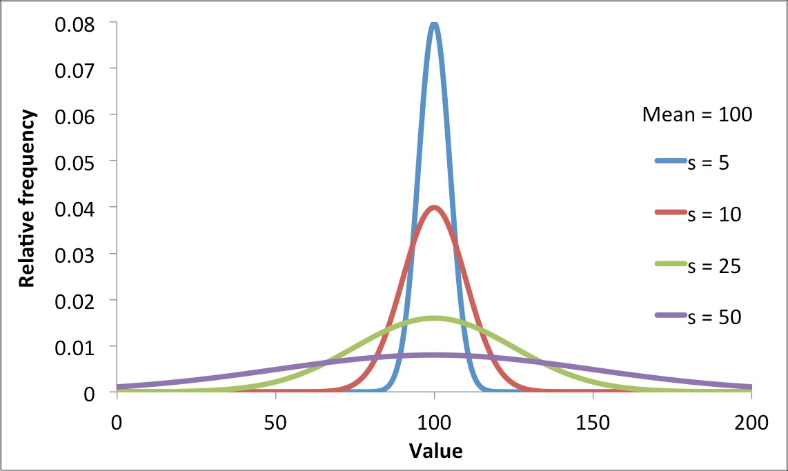
A normal distribution has a characteristic bell curve, but the midpoint and width of the curve varies between data sets. The width of the curve depends on the magnitude of the standard deviation. Figure 5 below shows how as the standard deviation increases, the curve becomes wider and shorter. A larger standard deviation indicates there are more measurements that lie relatively far from the mean. A smaller standard deviation characterizes a dataset that has the measurements closer to the mean. The dataset with the smaller standard deviation is said to be more precise. Standard deviation does not tell us about accuracy.

A normal distribution can also be thought of as a density function. The area under the curve is constant for all normal distributions as it is always equal to 1 (by definition). A key feature of a normal distribution is that the area defined by two values along the x-axis represents the probability of a randomly distributed measurement falling within that range. Figure 6 below shows the percentage of results that fall within one, two and three standard deviations of the mean. We can see that about 68% of measurements will fall within the range \(\bar{x}\) ± 1s, 95% of measurements will fall within \(\bar{x}\) ± 2s and 99.7% of measurements will fall within \(\bar{x}\) ± 3s. The probability of a measurement lying beyond ± three standard deviations is low.

In the case of Taconite Lake, for which 100 samples were taken and analyzed, a normal curve was produced. Using this normal curve, mean and standard deviation, the researchers could estimate the number of samples that are expected to lie within specific ranges. Figure 7 shows samples (represented by red dots) and the normal curve for the data.

Imagine the researchers wanted to estimate how many samples lie between concentrations 0.180 \(\mu\)g/L and 0.220 \(\mu\)g/L. This range is equal to two standard deviations on either side of the mean. From Figure 6, we know that ± two standard deviations corresponds to 95% of the total samples. This means that of the 100 samples, 95 should lie within this range.

In that example, we chose the numbers to reinforce to you that 95% of normally distributed data lies within 2 standard deviations of the mean, but you can imagine more scientifically relevant uses to this approach; in fact, the power of the normal distribution is it allows you to predict the probability that future measurement(s) will be in a particular range. Perhaps there is some dose of lead above which health concerns rise rapidly; we might then want to know what percentage of our water samples will be expected to measure above that concentration.

The Normal Distribution: Effects of Sample Size

As we discussed earlier, the more replicates measured, the better the mean approximates the true value. A set of data may be normally distributed, but it often requires a large number of samples to be able to see the pattern of the normal distribution. At smaller sample sizes, distributions of measured values usually do not have the nice bell-curved shape that defines a normal distribution (see Figure 8).

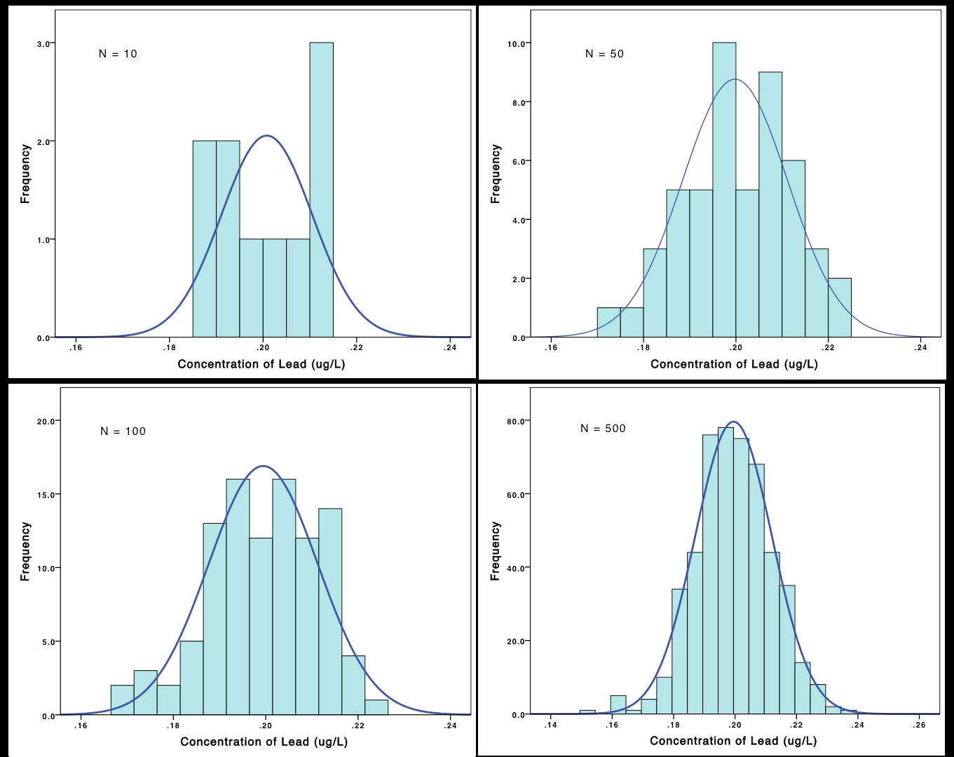
In Figure 8 it can be seen that as the number of samples increases, the histogram increasingly begins to resemble a normal distribution. Since measuring the concentration of lead in Taconite Lake is important for the health of the residents of the nearby town, it isn't unreasonable for hundreds of samples to be taken (measurements might be taken hourly or daily). But when working in a lab, it is often unreasonable to take hundreds of replicates to obtain the normal distribution. Thankfully, you probably already know that a normal distribution is not needed to determine the mean and standard deviation of a set of data.

Even though it isn't necessary to obtain a normal distribution with every set of samples, it can be important to know whether or not a sample would produce a normal distribution if many replicate measurements were made. Data that do not follow a normal distribution are treated with different statistical tests than data that produces normal distributions. It is rare in the natural sciences for measurements not to follow a normal distribution.